Excel Tip of the Week #431 - SUBSTITUTE redux

Basic SUBSTITUTE

The general idea of SUBSTITUTE is that it can be used to find a piece of text within a string, and replace it with another piece – similar to the classic find & replace, except with a formula rather than as an action. This means it can be reused more easily, and also doesn’t get rid of the input data, instead creating the transformed version in another cell.

Here’s a look at the syntax of this function:

=SUBSTITUTE(text, old text, new text, instance num)

Text is the original text string that you want to amend. This is most commonly just a reference to a single other cell, but could also be a formula that returns a text value.

Old text is the string that will be replaced. Again, this can be a cell reference or a formula – even just one like “a” that contains the old text in quote marks. Note that SUBSTITUTE is case-sensitive, so “a” and “A” are treated differently.

New text is what that old text will be replaced with – again, either a cell reference, a formula, or a direct entry with quote marks.

Instance num is an optional extra; if not included, every instance of the old text will be replaced. If an instance num value is provided, then only that instance will be replaced – so for example you could use a 1 to only replace the first instance of the old text.

Here’s a look at the formula in practice:

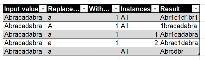
Note how the capital and lower-case As are treated differently. Also note how the last example shows you could also use a null (“”) or empty cell to simply remove the old text.

It’s worth noting that SUBSTITUTE is a text function, so whatever comes out of it will be a text value. If you’re using SUBSTITUTE to clean up numeric data, then you will need to use the VALUE function or multiply the result by 1 to convert it:

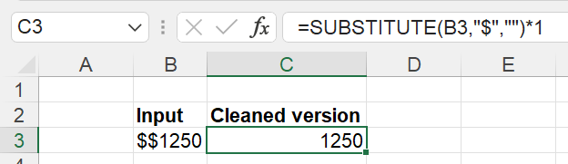
Note that if you want currency symbols applied to your final result, the correct way to do this is to create a clean number with a formula such as the above, and then apply a currency format. This displays the figure in the cell without including it in the actual value that is used in calculations.

Advanced SUBSTITUTE

There are a few extra tricks you can consider with SUBSTITUTE that can increase its usefulness.

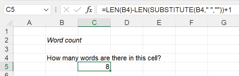
Word counting

There’s no inbuilt word count function in Excel, but you can use SUBSTITUTE to do one – compare the length of a text string with the length of that string after using SUBSTITUTE to remove all the spaces. The difference is the number of spaces; add 1 to get your word count:

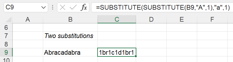
Changing multiple strings

We’ll look at some really advanced methods for this later, but for a basic approach, we can nest formulas, having one SUBSTITUTE function be the input to another:

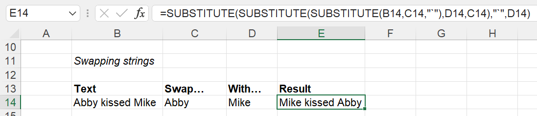
Swapping two strings

If you want to swap two strings over – replacing each with the other – then you need to use three SUBSTITUTE functions:

1. Change the first string to a dummy character that isn’t otherwise used (I like using the backtick character ` as it is easily typed and never really seen in text)
2. Change the second string to the first string
3. Change the dummy character to the second string

Don’t forget that formulas calculate from the inside outward!

Automating multiple substitutions

Finally – if you have a whole list of substitutions to make, how can you do it? Nesting SUBSTITUTE functions will only get you so far. If you want to systematically replace each of a list of strings with a corresponding list, you need to look into using VBA or (if you have the latest versions of Excel), the LAMBDA function to create your own function.

Here’s a VBA user-defined function that can do the job – see TOTW #410 for a how-to guide on how to install VBA if you don’t know how.

Public Function VBASUBALL(text As Range, oldtext As Range, newtext As Range) As String

 

Dim carrier As String
carrier = text

For i = 1 To oldtext.Count
    carrier = WorksheetFunction.Substitute(carrier, oldtext(i), newtext(i))
Next i

VBASUBALL = carrier

End Function

Or, if you have the LAMBDA function, you could write this as the definition for a defined name called SUBALL:

=LAMBDA(text, old, new, start, IF(start<=ROWS(old), SUBSTITUTE(SUBALL(text, old, new, start + 1), INDEX(old,start), INDEX(new, start)), text))

You can see examples of both of these in practice, along with all the other functions from today’s tip, in the accompanying file.

• Previous post - 3D maps
• TOTW index
• Next time – Date-creating formulas redux!